I memorized Kadane’s algorithm in college. I knew the code by heart: maxEndingHere = Math.max(num, maxEndingHere + num). I could write it on a whiteboard without thinking. But when someone asked me why it worked, I could not explain it. I just knew it did. That bothered me for years.
Kadane’s algorithm finds the maximum sum of any contiguous subarray in O(n). It is deceptively simple — four lines of code — but the insight behind it is a dynamic programming recurrence in disguise. Once you understand the insight, you stop memorizing and start deriving.
Short version: At each position, you have two choices: extend the previous subarray or start a new one. Pick whichever gives the larger sum. The maximum among all positions is the answer.
The Core Decision: Extend or Start Fresh
Imagine walking through an array from left to right. At each element, you hold the maximum sum you can achieve for a subarray ending at the previous position. When you arrive at the current element, you have exactly two options:
- Extend: Add the current element to the previous subarray. The new sum is
previousMax + current. - Start fresh: Discard the previous subarray and start a new one at the current element. The new sum is
current.
You pick whichever is larger. That is the entire algorithm.
The two variables handle different responsibilities. maxEndingHere tracks the best sum ending at the current position — it is the local optimum that gets updated at every step. maxSoFar tracks the best sum seen anywhere so far — it is the global optimum that only updates when the local optimum beats the previous record. The Math.max call inside the loop implements the decision: if extending produces a larger sum, keep going. If starting fresh is better, abandon the previous subarray entirely.
Most developers who have seen Kadane can recite these four lines. The part that takes time to internalize is that this simple decision rule is sufficient. There is no need to check all possible subarrays, no need to compare against a threshold, no need to look ahead at future elements. The local decision at each position, combined with tracking the maximum across all positions, produces the correct global answer.
function maxSubarray(nums) {
  let maxEndingHere = nums[0]
  let maxSoFar = nums[0]
  for (let i = 1; i < nums.length; i++) {
    maxEndingHere = Math.max(nums[i], maxEndingHere + nums[i])
    maxSoFar = Math.max(maxSoFar, maxEndingHere)
  }
  return maxSoFar
}
Let’s trace through what this code does. It starts by assuming the first element is both the local best and the global best. Then for each subsequent element, it asks: is this element valuable enough to extend the current subarray, or would it be better to discard everything and start fresh from here? The Math.max call answers that question. If the current element alone is larger than the current subarray plus the element, the previous subarray was dragging the sum down and gets thrown away. The global maximum is updated whenever the local best exceeds the previous record.
This pattern of updating a local candidate and comparing it against a global best appears in many optimization algorithms. Understanding why this simple loop works without any backtracking is the key to understanding Kadane fully.
The decision flow below traces how the algorithm chooses between extending and restarting at each step. The yellow diamond highlights the critical reset moment where starting fresh beats extending.
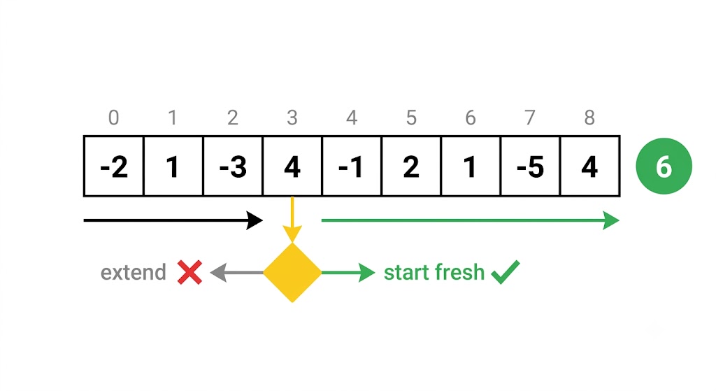
The flowchart above shows the decision process. At each position, the algorithm evaluates two paths: keep extending the current subarray or abandon it and start fresh. The yellow diamond at index 3 is the critical moment where extending would produce a smaller sum than restarting. After that, extending is always the better choice.
Walking Through an Example
Take the array [-2, 1, -3, 4, -1, 2, 1, -5, 4]. At index 0, maxEndingHere = -2, maxSoFar = -2. At index 1, the value is 1. Extending would give -1. Starting fresh gives 1. You pick 1. At index 2, the value is -3. Extending gives -2. Starting fresh gives -3. Extending is less bad.
At index 3, the value is 4. Extending gives 2. Starting fresh gives 4. You pick 4. This is the key moment: the algorithm resets because the previous sum was negative. It recognizes that carrying a negative sum forward reduces the total, so it starts a new subarray. From there, extending is always better. The subarray [4, -1, 2, 1] sums to 6, which becomes the final answer.
The algorithm never looks back. It never backtracks or scans ahead. Each element is visited exactly once and either starts a new subarray or extends the current one. The table below shows every step for this example clearly.
| Index | Value | Extend | Start Fresh | Choose | Best So Far |
|---|---|---|---|---|---|
| 0 | -2 | - | -2 | -2 | -2 |
| 1 | 1 | -1 | 1 | 1 | 1 |
| 2 | -3 | -2 | -3 | -2 | 1 |
| 3 | 4 | 2 | 4 | 4 | 4 |
| 4 | -1 | 3 | -1 | 3 | 4 |
| 5 | 2 | 5 | 2 | 5 | 5 |
| 6 | 1 | 6 | 1 | 6 | 6 |
| 7 | -5 | 1 | -5 | 1 | 6 |
| 8 | 4 | 5 | 4 | 5 | 6 |
Notice how the “Start Fresh” column wins only once — at index 3, where the value 4 resets the algorithm. After that, extending always produces a better sum than starting fresh. The “Best So Far” column updates whenever the current sum exceeds the previous maximum, which happens at index 3 and index 6.
Why It Is a DP Problem
Kadane’s algorithm is dynamic programming in disguise. If you expand the code into an explicit DP table, the recurrence relation becomes clear: dp[i] = max(nums[i], dp[i-1] + nums[i]), where dp[i] is the maximum subarray sum ending at index i. The final answer is the maximum value in the entire dp array.
The full DP version makes this structure explicit:
function maxSubarrayDP(nums) {
  const dp = [nums[0]]
  for (let i = 1; i < nums.length; i++) {
    dp[i] = Math.max(nums[i], dp[i-1] + nums[i])
  }
  return Math.max(...dp)
}
The difference between the full DP version and Kadane becomes clearer when you see how the running sum changes across the array. A single pass tracks both the local and global maximum, and this visualization shows the exact moment the algorithm resets.
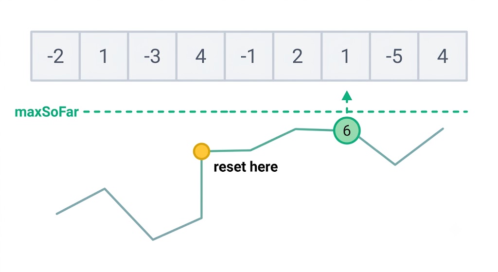
The line graph above visualizes how the running sum evolves. The sharp jump at index 3 marks the reset point where the algorithm discards the negative prefix and starts fresh. The peak at index 6 shows where the maximum subarray sum of 6 is achieved. The horizontal dashed line tracks the best value seen so far.
This version allocates an array, fills it from left to right, and each cell depends only on the previous cell. Kadane’s optimization is to notice that you never need the entire array. At step i, you only need dp[i-1] to compute dp[i]. All earlier values can be discarded. This reduces memory from O(n) to O(1).
This space optimization pattern appears across many classic DP problems. In Fibonacci, you only need the last two values instead of the full sequence. In climbing stairs, you only need the previous two step counts. In the house robber problem, you only need the maximum up to the previous two houses. Recognizing when a full DP table can be replaced with a rolling variable is a skill that transfers directly from Kadane to more complex problems.
Kadane appears in almost every DP curriculum because it is the simplest complete example of the entire DP workflow: define a recurrence, implement with a table, then optimize space. Once you understand Kadane, you understand the template for solving dozens of other DP problems.
Local Decisions, Global Optimum
This is the most surprising part. At each position, you make a local decision: extend or restart. You have no information about future elements. Yet the maximum among all local decisions is guaranteed to be the global maximum. This works because the optimal subarray must end somewhere. At that ending position, the local decision will necessarily pick the extension because the sum up to that point is the maximum possible. The algorithm finds the optimal subarray without knowing its start position in advance. It does not need to know where the optimal subarray starts; it only needs to recognize it when it reaches its end.
This property is not unique to Kadane. It applies to any problem where the optimal solution can be built from optimal solutions to smaller subproblems. That is the defining characteristic of dynamic programming. Kadane is just the cleanest example of this principle, which is why understanding it deeply makes every other DP problem easier to reason about.